参考答案

python

import numpy as np
import pandas as pd
import matplotlib.pyplot as plt

第一章预备知识

Ex1：利用列表推导式写矩阵乘法

python

M1 = np.random.rand(2,3)
M2 = np.random.rand(3,4)
res = [[sum([M1[i][k] * M2[k][j] for k in range(M1.shape[1])]) for j in range(M2.shape[1])] for i in range(M1.shape[0])]
(np.abs((M1@M2 - res) < 1e-15)).all()

True

Ex2：更新矩阵

python

A = np.arange(1,10).reshape(3,-1)
B = A*(1/A).sum(1).reshape(-1,1)
B

array([[1.83333333, 3.66666667, 5.5       ],
       [2.46666667, 3.08333333, 3.7       ],
       [2.65277778, 3.03174603, 3.41071429]])

Ex3：卡方统计量

python

np.random.seed(0)
A = np.random.randint(10, 20, (8, 5))
B = A.sum(0)*A.sum(1).reshape(-1, 1)/A.sum()
res = ((A-B)**2/B).sum()
res

11.842696601945802

Ex4：改进矩阵计算的性能

原方法：

python

np.random.seed(0)
m, n, p = 100, 80, 50
B = np.random.randint(0, 2, (m, p))
U = np.random.randint(0, 2, (p, n))
Z = np.random.randint(0, 2, (m, n))
def solution(B=B, U=U, Z=Z):
    L_res = []
    for i in range(m):
        for j in range(n):
            norm_value = ((B[i]-U[:,j])**2).sum()
            L_res.append(norm_value*Z[i][j])
    return sum(L_res)
solution(B, U, Z)

改进方法：

令 $Y_{i j} = ∥ B_{i} - U_{j} ∥_{2}^{2}$ ，则 $R = \sum_{i = 1}^{m} \sum_{j = 1}^{n} Y_{i j} Z_{i j}$ ，这在Numpy中可以用逐元素的乘法后求和实现，因此问题转化为了如何构造Y矩阵。

\begin{aligned} Y_{i j} & = ∥ B_{i} - U_{j} ∥_{2}^{2} \\ = \sum_{k = 1}^{p} (B_{i k} - U_{k j})^{2} \\ = \sum_{k = 1}^{p} B_{i k}^{2} + \sum_{k = 1}^{p} U_{k j}^{2} - 2 \sum_{k = 1}^{p} B_{i k} U_{k j} \end{aligned}

从上式可以看出，第一第二项分别为 $B$ 的行平方和与 $U$ 的列平方和，第三项是两倍的内积。因此， $Y$ 矩阵可以写为三个部分，第一个部分是 $m \times n$ 的全 $1$ 矩阵每行乘以 $B$ 对应行的行平方和，第二个部分是相同大小的全 $1$ 矩阵每列乘以 $U$ 对应列的列平方和，第三个部分恰为 $B$ 矩阵与 $U$ 矩阵乘积的两倍。从而结果如下：

python

(((B**2).sum(1).reshape(-1,1) + (U**2).sum(0) - 2*B@U)*Z).sum()

对比它们的性能：

python

%timeit -n 30 solution(B, U, Z)

48.5 ms ± 4.39 ms per loop (mean ± std. dev. of 7 runs, 30 loops each)

python

%timeit -n 30 ((np.ones((m,n))*(B**2).sum(1).reshape(-1,1) + np.ones((m,n))*(U**2).sum(0) - 2*B@U)*Z).sum()

1.11 ms ± 47 µs per loop (mean ± std. dev. of 7 runs, 30 loops each)

Ex5：连续整数的最大长度

python

f = lambda x:np.diff(np.nonzero(np.r_[1,np.diff(x)!=1,1])).max()
f([1,2,5,6,7])
f([3,2,1,2,3,4,6])

第二章 pandas基础

Ex1：口袋妖怪数据集

1.

python

df = pd.read_csv('../data/pokemon.csv')
(df[['HP', 'Attack', 'Defense', 'Sp. Atk', 'Sp. Def', 'Speed']].sum(1)!=df['Total']).mean()

0.0

2.

(a)

python

dp_dup = df.drop_duplicates('#', keep='first')
dp_dup['Type 1'].nunique()
dp_dup['Type 1'].value_counts().index[:3]

Index(['Water', 'Normal', 'Grass'], dtype='object')

(b)

python

attr_dup = dp_dup.drop_duplicates(['Type 1', 'Type 2'])
attr_dup.shape[0]

(c)

python

L_full = [i+' '+j if i!=j else i for i in df['Type 1'].unique() for j in df['Type 1'].unique()]
L_part = [i+' '+j if not isinstance(j, float) else i for i, j in zip(df['Type 1'], df['Type 2'])]
res = set(L_full).difference(set(L_part))
len(res) # 太多，不打印了

3.

(a)

python

df['Attack'].mask(df['Attack']>120, 'high').mask(df['Attack']<50, 'low').mask((50<=df['Attack'])&(df['Attack']<=120), 'mid').head()

0    low
1    mid
2    mid
3    mid
4    mid
Name: Attack, dtype: object

(b)

python

df['Type 1'].replace({i:str.upper(i) for i in df['Type 1'].unique()})
df['Type 1'].apply(lambda x:str.upper(x)).head()

0    GRASS
1    GRASS
2    GRASS
3    GRASS
4     FIRE
Name: Type 1, dtype: object

(c)

python

df['Deviation'] = df[['HP', 'Attack', 'Defense', 'Sp. Atk', 'Sp. Def', 'Speed']].apply(lambda x:np.max((x-x.median()).abs()), 1)
df.sort_values('Deviation', ascending=False).head()

	#	Name	Type 1	Type 2	Total	HP	Attack	Defense	Sp. Atk	Sp. Def	Speed	Deviation
230	213	Shuckle	Bug	Rock	505	20	10	230	10	230	5	215.0
121	113	Chansey	Normal	NaN	450	250	5	5	35	105	50	207.5
261	242	Blissey	Normal	NaN	540	255	10	10	75	135	55	190.0
333	306	AggronMega Aggron	Steel	NaN	630	70	140	230	60	80	50	155.0
224	208	SteelixMega Steelix	Steel	Ground	610	75	125	230	55	95	30	145.0

Ex2：指数加权窗口

1.

python

np.random.seed(0)
s = pd.Series(np.random.randint(-1,2,30).cumsum())
s.ewm(alpha=0.2).mean().head()
def ewm_func(x, alpha=0.2):
    win = (1-alpha)**np.arange(x.shape[0])[::-1]
    res = (win*x).sum()/win.sum()
    return res
s.expanding().apply(ewm_func).head()

0   -1.000000
1   -1.000000
2   -1.409836
3   -1.609756
4   -1.725845
dtype: float64

2.

新的权重为 $w_{i} = (1 - α)^{i}, i \in {0, 1, . . ., n - 1}$ ， $y_{t}$ 更新如下：

\begin{aligned} y_{t} & = \frac{\sum_{i = 0}^{n - 1} w_{i} x_{t - i}}{\sum_{i = 0}^{n - 1} w_{i}} \\ = \frac{x_{t} + (1 - α) x_{t - 1} + (1 - α)^{2} x_{t - 2} + . . . + (1 - α)^{n - 1} x_{t - (n - 1)}}{1 + (1 - α) + (1 - α)^{2} + . . . + (1 - α)^{n - 1}} \end{aligned}

python

s.rolling(window=4).apply(ewm_func).head() # 无需对原函数改动

0         NaN
1         NaN
2         NaN
3   -1.609756
4   -1.826558
dtype: float64

第三章索引

Ex1：公司员工数据集

1.

python

df = pd.read_csv('../data/company.csv')
dpt = ['Dairy', 'Bakery']
df.query("(age <= 40)&(department == @dpt)&(gender=='M')").head(3)

	EmployeeID	birthdate_key	age	city_name	department	job_title	gender
3611	5791	1/14/1975	40	Kelowna	Dairy	Dairy Person	M
3613	5793	1/22/1975	40	Richmond	Bakery	Baker	M
3615	5795	1/30/1975	40	Nanaimo	Dairy	Dairy Person	M

python

df.loc[(df.age<=40)&df.department.isin(dpt)&(df.gender=='M')].head(3)

	EmployeeID	birthdate_key	age	city_name	department	job_title	gender
3611	5791	1/14/1975	40	Kelowna	Dairy	Dairy Person	M
3613	5793	1/22/1975	40	Richmond	Bakery	Baker	M
3615	5795	1/30/1975	40	Nanaimo	Dairy	Dairy Person	M

2.

python

df.iloc[(df.EmployeeID%2==1).values,[0,2,-2]].head()

	EmployeeID	age	job_title
1	1319	58	VP Stores
3	1321	56	VP Human Resources
5	1323	53	Exec Assistant, VP Stores
6	1325	51	Exec Assistant, Legal Counsel
8	1329	48	Store Manager

3.

python

df_op = df.copy()
df_op = df_op.set_index(df_op.columns[-3:].tolist()).swaplevel(0,2,axis=0)
df_op = df_op.reset_index(level=1)
df_op = df_op.rename_axis(index={'gender':'Gender'})
df_op.index = df_op.index.map(lambda x:'_'.join(x))
df_op.index = df_op.index.map(lambda x:tuple(x.split('_')))
df_op = df_op.rename_axis(index=['gender', 'department'])
df_op = df_op.reset_index().reindex(df.columns, axis=1)
df_op.equals(df)

True

Ex2：巧克力数据集

1.

python

df = pd.read_csv('../data/chocolate.csv')
df.columns = [' '.join(i.split('\n')) for i in df.columns]
df.head(3)

	Company	Review Date	Cocoa Percent	Company Location	Rating
0	A. Morin	2016	63%	France	3.75
1	A. Morin	2015	70%	France	2.75
2	A. Morin	2015	70%	France	3.00

2.

python

df['Cocoa Percent'] = df['Cocoa Percent'].apply(lambda x:float(x[:-1])/100)
df.query('(Rating<3)&(`Cocoa Percent`>`Cocoa Percent`.median())').head(3)

	Company	Review Date	Cocoa Percent	Company Location	Rating
33	Akesson's (Pralus)	2010	0.75	Switzerland	2.75
34	Akesson's (Pralus)	2010	0.75	Switzerland	2.75
36	Alain Ducasse	2014	0.75	France	2.75

3.

python

idx = pd.IndexSlice
exclude = ['France', 'Canada', 'Amsterdam', 'Belgium']
res = df.set_index(['Review Date', 'Company Location']).sort_index(level=0)
res.loc[idx[2012:,~res.index.get_level_values(1).isin(exclude)],:].head(3)

		Company	Cocoa Percent	Rating
Review Date	Company Location
2012	Australia	Bahen & Co.	0.7	3.0
	Australia	Bahen & Co.	0.7	2.5
	Australia	Bahen & Co.	0.7	2.5

第四章分组

Ex1：汽车数据集

1.

python

df = pd.read_csv('../data/car.csv')
df.groupby('Country').filter(lambda x:x.shape[0]>2).groupby('Country')['Price'].agg([('CoV', lambda x: x.std()/x.mean()), 'mean', 'count'])

	CoV	mean	count
Country
Japan	0.387429	13938.052632	19
Japan/USA	0.240040	10067.571429	7
Korea	0.243435	7857.333333	3
USA	0.203344	12543.269231	26

2.

python

df.shape[0]

python

condition = ['Head']*20+['Mid']*20+['Tail']*20
df.groupby(condition)['Price'].mean()

Head     9069.95
Mid     13356.40
Tail    15420.65
Name: Price, dtype: float64

3.

python

res = df.groupby('Type').agg({'Price': ['max'], 'HP': ['min']})
res.columns = res.columns.map(lambda x:'_'.join(x))
res

	Price_max	HP_min
Type
Compact	18900	95
Large	17257	150
Medium	24760	110
Small	9995	63
Sporty	13945	92
Van	15395	106

4.

python

def normalize(s):
    s_min, s_max = s.min(), s.max()
    res = (s - s_min)/(s_max - s_min)
    return res
df.groupby('Type')['HP'].transform(normalize).head()

0    1.00
1    0.54
2    0.00
3    0.58
4    0.80
Name: HP, dtype: float64

5.

python

df.groupby('Type')[['HP', 'Disp.']].apply(lambda x:np.corrcoef(x['HP'].values, x['Disp.'].values)[0,1])

Type
Compact    0.586087
Large     -0.242765
Medium     0.370491
Small      0.603916
Sporty     0.871426
Van        0.819881
dtype: float64

Ex2：实现transform函数

python

class my_groupby:
    def __init__(self, my_df, group_cols):
        self.my_df = my_df.copy()
        self.groups = my_df[group_cols].drop_duplicates()
        if isinstance(self.groups, pd.Series):
            self.groups = self.groups.to_frame()
        self.group_cols = self.groups.columns.tolist()
        self.groups = {i: self.groups[i].values.tolist() for i in self.groups.columns}
        self.transform_col = None
    def __getitem__(self, col):
        self.pr_col = [col] if isinstance(col, str) else list(col)
        return self
    def transform(self, my_func):
        self.num = len(self.groups[self.group_cols[0]])
        L_order, L_value = np.array([]), np.array([])
        for i in range(self.num):
            group_df = self.my_df.reset_index().copy()
            for col in self.group_cols:
                group_df = group_df[group_df[col]==self.groups[col][i]]
            group_df = group_df[self.pr_col]
            if group_df.shape[1] == 1:
                group_df = group_df.iloc[:, 0]
            group_res = my_func(group_df)
            if not isinstance(group_res, pd.Series):
                group_res = pd.Series(group_res,index=group_df.index,name=group_df.name)
            L_order = np.r_[L_order, group_res.index]
            L_value = np.r_[L_value, group_res.values]
        self.res = pd.Series(pd.Series(L_value, index=L_order).sort_index().values,index=self.my_df.reset_index().index, name=my_func.__name__)
        return self.res

my_groupby(df, 'Type')

<__main__.my_groupby at 0x1817feca9a0>

单列分组：

python

def f(s):
    res = (s-s.min())/(s.max()-s.min())
    return res
my_groupby(df, 'Type')['Price'].transform(f).head()

0    0.733592
1    0.372003
2    0.109712
3    0.186244
4    0.177525
Name: f, dtype: float64

python

df.groupby('Type')['Price'].transform(f).head()

0    0.733592
1    0.372003
2    0.109712
3    0.186244
4    0.177525
Name: Price, dtype: float64

多列分组：

python

my_groupby(df, ['Type','Country'])['Price'].transform(f).head()

0    1.000000
1    0.000000
2    0.000000
3    0.000000
4    0.196357
Name: f, dtype: float64

python

df.groupby(['Type','Country'])['Price'].transform(f).head()

0    1.000000
1    0.000000
2    0.000000
3    0.000000
4    0.196357
Name: Price, dtype: float64

标量广播：

python

my_groupby(df, 'Type')['Price'].transform(lambda x:x.mean()).head()

0    7682.384615
1    7682.384615
2    7682.384615
3    7682.384615
4    7682.384615
Name: <lambda>, dtype: float64

python

df.groupby('Type')['Price'].transform(lambda x:x.mean()).head()

0    7682.384615
1    7682.384615
2    7682.384615
3    7682.384615
4    7682.384615
Name: Price, dtype: float64

跨列计算：

python

my_groupby(df, 'Type')['Disp.', 'HP'].transform(lambda x: x['Disp.']/x.HP).head()

0    0.858407
1    1.266667
2    1.285714
3    0.989130
4    1.097087
Name: <lambda>, dtype: float64

第五章变形

Ex1：美国非法药物数据集

1.

python

df = pd.read_csv('../data/drugs.csv').sort_values(['State','COUNTY','SubstanceName'],ignore_index=True)
res = df.pivot(index=['State','COUNTY','SubstanceName'], columns='YYYY', values='DrugReports').reset_index().rename_axis(columns={'YYYY':''})
res.head(5)

	State	COUNTY	SubstanceName	2010	2011	2012	2013	2014	2015	2016	2017
0	KY	ADAIR	Buprenorphine	NaN	3.0	5.0	4.0	27.0	5.0	7.0	10.0
1	KY	ADAIR	Codeine	NaN	NaN	1.0	NaN	NaN	NaN	NaN	1.0
2	KY	ADAIR	Fentanyl	NaN	NaN	1.0	NaN	NaN	NaN	NaN	NaN
3	KY	ADAIR	Heroin	NaN	NaN	1.0	2.0	NaN	1.0	NaN	2.0
4	KY	ADAIR	Hydrocodone	6.0	9.0	10.0	10.0	9.0	7.0	11.0	3.0

2.

python

res_melted = res.melt(id_vars = ['State','COUNTY','SubstanceName'],
                      value_vars = res.columns[-8:],
                      var_name = 'YYYY',
                      value_name = 'DrugReports').dropna(
                      subset=['DrugReports'])
res_melted = res_melted[df.columns].sort_values(['State','COUNTY','SubstanceName'],ignore_index=True).astype({'YYYY':'int64', 'DrugReports':'int64'})
res_melted.equals(df)

True

3.

策略一：

python

res = df.pivot_table(index='YYYY', columns='State', values='DrugReports', aggfunc='sum')
res.head(3)

State	KY	OH	PA	VA	WV
YYYY
2010	10453	19707	19814	8685	2890
2011	10289	20330	19987	6749	3271
2012	10722	23145	19959	7831	3376

策略二：

python

res = df.groupby(['State', 'YYYY'])['DrugReports'].sum().to_frame().unstack(0).droplevel(0,axis=1)
res.head(3)

State	KY	OH	PA	VA	WV
YYYY
2010	10453	19707	19814	8685	2890
2011	10289	20330	19987	6749	3271
2012	10722	23145	19959	7831	3376

Ex2：特殊的wide_to_long方法

python

df = pd.DataFrame({'Class':[1,2],
                   'Name':['San Zhang', 'Si Li'],
                   'Chinese':[80, 90],
                   'Math':[80, 75]})
df

	Class	Name	Chinese	Math
0	1	San Zhang	80	80
1	2	Si Li	90	75

python

df = df.rename(columns={'Chinese':'pre_Chinese', 'Math':'pre_Math'})
pd.wide_to_long(df,
                stubnames=['pre'],
                i = ['Class', 'Name'],
                j='Subject',
                sep='_',
                suffix='.+').reset_index().rename(columns={'pre':'Grade'})

	Class	Name	Subject	Grade
0	1	San Zhang	Chinese	80
1	1	San Zhang	Math	80
2	2	Si Li	Chinese	90
3	2	Si Li	Math	75

第六章连接

Ex1：美国疫情数据集

python

date = pd.date_range('20200412', '20201116').to_series()
date = date.dt.month.astype('string').str.zfill(2) +'-'+ date.dt.day.astype('string').str.zfill(2) +'-'+ '2020'
date = date.tolist()

python

L = []
for d in date:
    df = pd.read_csv('../data/us_report/' + d + '.csv', index_col='Province_State')
    data = df.loc['New York', ['Confirmed','Deaths','Recovered','Active']]
    L.append(data.to_frame().T)
res = pd.concat(L)
res.index = date
res.head()

	Confirmed	Deaths	Recovered	Active
04-12-2020	189033	9385	23887.0	179648
04-13-2020	195749	10058	23887.0	185691.0
04-14-2020	203020	10842	23887.0	192178.0
04-15-2020	214454	11617	23887.0	202837.0
04-16-2020	223691	14832	23887.0	208859.0

Ex2：实现join函数

python

def join(df1, df2, how='left'):
    res_col = df1.columns.tolist() +  df2.columns.tolist()
    dup = df1.index.unique().intersection(df2.index.unique())
    res_df = pd.DataFrame(columns = res_col)
    for label in dup:
        cartesian = [list(i)+list(j) for i in df1.loc[label].values.reshape(-1,1) for j in df2.loc[label].values.reshape(-1,1)]
        dup_df = pd.DataFrame(cartesian, index = [label]*len(cartesian), columns = res_col)
        res_df = pd.concat([res_df,dup_df])
    if how in ['left', 'outer']:
        for label in df1.index.unique().difference(dup):
            if isinstance(df1.loc[label], pd.DataFrame):
                cat = [list(i)+[np.nan]*df2.shape[1] for i in df1.loc[label].values]
            else:
                cat = [list(i)+[np.nan]*df2.shape[1] for i in df1.loc[label].to_frame().values]
            dup_df = pd.DataFrame(cat, index = [label]*len(cat), columns = res_col)
            res_df = pd.concat([res_df,dup_df])
    if how in ['right', 'outer']:
        for label in df2.index.unique().difference(dup):
            if isinstance(df2.loc[label], pd.DataFrame):
                cat = [[np.nan]+list(i)*df1.shape[1] for i in df2.loc[label].values]
            else:
                cat = [[np.nan]+list(i)*df1.shape[1] for i in df2.loc[label].to_frame().values]
            dup_df = pd.DataFrame(cat, index = [label]*len(cat), columns = res_col)
            res_df = pd.concat([res_df,dup_df])
    return res_df

python

df1 = pd.DataFrame({'col1':[1,2,3,4,5]}, index=list('AABCD'))
df1

	col1
A	1
A	2
B	3
C	4
D	5

python

df2 = pd.DataFrame({'col2':list('opqrst')}, index=list('ABBCEE'))
df2

	col2
A	o
B	p
B	q
C	r
E	s
E	t

python

join(df1, df2, how='inner')

	col1	col2
A	1	o
A	2	o
B	3	p
B	3	q
C	4	r

第七章缺失数据

Ex1：缺失值与类别的相关性检验

python

df = pd.read_csv('../data/missing_chi.csv')
cat_1 = df.X_1.fillna('NaN').mask(df.X_1.notna()).fillna("NotNaN")
cat_2 = df.X_2.fillna('NaN').mask(df.X_2.notna()).fillna("NotNaN")
df_1 = pd.crosstab(cat_1, df.y, margins=True)
df_2 = pd.crosstab(cat_2, df.y, margins=True)
def compute_S(my_df):
    S = []
    for i in range(2):
        for j in range(2):
            E = my_df.iat[i, j]
            F = my_df.iat[i, 2]*my_df.iat[2, j]/my_df.iat[2,2]
            S.append((E-F)**2/F)
    return sum(S)
res1 = compute_S(df_1)
res2 = compute_S(df_2)
from scipy.stats import chi2
chi2.sf(res1, 1) # X_1检验的p值 # 不能认为相关，剔除

0.9712760884395901

python

chi2.sf(res2, 1) # X_2检验的p值 # 认为相关，保留

7.459641265637543e-166

结果与scipy.stats.chi2_contingency在不使用 $Y a t e s$ 修正的情况下完全一致：

python

from scipy.stats import chi2_contingency
chi2_contingency(pd.crosstab(cat_1, df.y), correction=False)[1]
chi2_contingency(pd.crosstab(cat_2, df.y), correction=False)[1]

7.459641265637543e-166

Ex2：用回归模型解决分类问题

1.

python

from sklearn.neighbors import KNeighborsRegressor
df = pd.read_excel('../data/color.xlsx')
df_dummies = pd.get_dummies(df.Color)
stack_list = []
for col in df_dummies.columns:
    clf = KNeighborsRegressor(n_neighbors=6)
    clf.fit(df.iloc[:,:2], df_dummies[col])
    res = clf.predict([[0.8, -0.2]]).reshape(-1,1)
    stack_list.append(res)
code_res = pd.Series(np.hstack(stack_list).argmax(1))
df_dummies.columns[code_res[0]]

c:\Users\gyh\miniconda3\envs\jp\lib\site-packages\sklearn\base.py:450: UserWarning: X does not have valid feature names, but KNeighborsRegressor was fitted with feature names
  warnings.warn(
c:\Users\gyh\miniconda3\envs\jp\lib\site-packages\sklearn\base.py:450: UserWarning: X does not have valid feature names, but KNeighborsRegressor was fitted with feature names
  warnings.warn(
c:\Users\gyh\miniconda3\envs\jp\lib\site-packages\sklearn\base.py:450: UserWarning: X does not have valid feature names, but KNeighborsRegressor was fitted with feature names
  warnings.warn(





'Yellow'

2.

python

from sklearn.neighbors import KNeighborsRegressor
df = pd.read_csv('../data/audit.csv')
res_df = df.copy()
df = pd.concat([pd.get_dummies(df[['Marital', 'Gender']]), df[['Age','Income','Hours']].apply(lambda x:(x-x.min())/(x.max()-x.min())), df.Employment],1)
X_train = df.query('Employment.notna()')
X_test = df.query('Employment.isna()')
df_dummies = pd.get_dummies(X_train.Employment)
stack_list = []
for col in df_dummies.columns:
    clf = KNeighborsRegressor(n_neighbors=6)
    clf.fit(X_train.iloc[:,:-1], df_dummies[col])
    res = clf.predict(X_test.iloc[:,:-1]).reshape(-1,1)
    stack_list.append(res)
code_res = pd.Series(np.hstack(stack_list).argmax(1))
cat_res = code_res.replace(dict(zip(list(range(df_dummies.shape[0])),df_dummies.columns)))
res_df.loc[res_df.Employment.isna(), 'Employment'] = cat_res.values
res_df.isna().sum()

ID            0
Age           0
Employment    0
Marital       0
Income        0
Gender        0
Hours         0
dtype: int64

第八章文本数据

Ex1：房屋信息数据集

1.

python

df = pd.read_excel('../data/house_info.xls', usecols=['floor','year','area','price'])
df.year = pd.to_numeric(df.year.str[:-2]).astype('Int64')
df.head(3)

	floor	year	area	price
0	高层（共6层）	1986	58.23㎡	155万
1	中层（共20层）	2020	88㎡	155万
2	低层（共28层）	2010	89.33㎡	365万

2.

python

pat = '(\w层)（共(\d+)层）'
new_cols = df.floor.str.extract(pat).rename(columns={0:'Level', 1:'Highest'})
df = pd.concat([df.drop(columns=['floor']), new_cols], 1)
df.head(3)

	year	area	price	Level	Highest
0	1986	58.23㎡	155万	高层	6
1	2020	88㎡	155万	中层	20
2	2010	89.33㎡	365万	低层	28

3.

python

s_area = pd.to_numeric(df.area.str[:-1])
s_price = pd.to_numeric(df.price.str[:-1])
df['avg_price'] = ((s_price/s_area)*10000).astype('int').astype('string') + '元/平米'
df.head(3)

	year	area	price	Level	Highest	avg_price
0	1986	58.23㎡	155万	高层	6	26618元/平米
1	2020	88㎡	155万	中层	20	17613元/平米
2	2010	89.33㎡	365万	低层	28	40859元/平米

Ex2：《权力的游戏》剧本数据集

1.

python

df = pd.read_csv('../data/script.csv')
df.columns = df.columns.str.strip()
df.groupby(['Season', 'Episode'])['Sentence'].count().head()

Season    Episode   
Season 1  Episode 1     327
          Episode 10    266
          Episode 2     283
          Episode 3     353
          Episode 4     404
Name: Sentence, dtype: int64

2.

python

df.set_index('Name').Sentence.str.split().str.len().groupby('Name').mean().sort_values(ascending=False).head()

Name
male singer          109.000000
slave owner           77.000000
manderly              62.000000
lollys stokeworth     62.000000
dothraki matron       56.666667
Name: Sentence, dtype: float64

3.

python

s = pd.Series(df.Sentence.values, index=df.Name.shift(-1))
s.str.count('\?').groupby('Name').sum().sort_values(ascending=False).head()

Name
tyrion lannister    527
jon snow            374
jaime lannister     283
arya stark          265
cersei lannister    246
dtype: int64

第九章分类数据

Ex1：统计未出现的类别

python

def my_crosstab(s1, s2, dropna=True):
    idx1 = (s1.cat.categories if s1.dtype.name == 'category' and not dropna else s1.unique())
    idx2 = (s2.cat.categories if s2.dtype.name == 'category' and not dropna else s2.unique())
    res = pd.DataFrame(np.zeros((idx1.shape[0], idx2.shape[0])), index=idx1, columns=idx2)
    for i, j in zip(s1, s2):
        res.at[i, j] += 1
    res = res.rename_axis(index=s1.name, columns=s2.name).astype('int')
    return res
df = pd.DataFrame({'A':['a','b','c','a'], 'B':['cat','cat','dog','cat']})
df.B = df.B.astype('category').cat.add_categories('sheep')
my_crosstab(df.A, df.B)
my_crosstab(df.A, df.B, dropna=False)

B	cat	dog	sheep
A
a	2	0	0
b	1	0	0
c	0	1	0

Ex2：钻石数据集

1.

python

df = pd.read_csv('../data/diamonds.csv')
s_obj, s_cat = df.cut, df.cut.astype('category')

python

%timeit -n 30 s_obj.nunique()

9.31 ms ± 756 µs per loop (mean ± std. dev. of 7 runs, 30 loops each)

python

%timeit -n 30 s_cat.nunique()

1.97 ms ± 156 µs per loop (mean ± std. dev. of 7 runs, 30 loops each)

2.

python

df.cut = df.cut.astype('category').cat.reorder_categories(['Fair', 'Good', 'Very Good', 'Premium', 'Ideal'],ordered=True)
df.clarity = df.clarity.astype('category').cat.reorder_categories(['I1', 'SI2', 'SI1', 'VS2', 'VS1', 'VVS2', 'VVS1', 'IF'],ordered=True)
res = df.sort_values(['cut', 'clarity'], ascending=[False, True])
res.head(3)

	carat	cut	clarity	price
315	0.96	Ideal	I1	2801
535	0.96	Ideal	I1	2826
551	0.97	Ideal	I1	2830

python

res.tail(3)

	carat	cut	clarity	price
47407	0.52	Fair	IF	1849
49683	0.52	Fair	IF	2144
50126	0.47	Fair	IF	2211

3.

python

df.cut = df.cut.cat.reorder_categories(df.cut.cat.categories[::-1])
df.clarity = df.clarity.cat.reorder_categories(df.clarity.cat.categories[::-1])

python

df.cut = df.cut.cat.codes # 方法一：利用cat.codes

python

clarity_cat = df.clarity.cat.categories
df.clarity = df.clarity.replace(dict(zip(clarity_cat, np.arange(len(clarity_cat))))) # 方法二：使用replace映射

python

df.head(3)

	carat	cut	clarity	price
0	0.23	0	6	326
1	0.21	1	5	326
2	0.23	3	3	327

4.

python

q = [0, 0.2, 0.4, 0.6, 0.8, 1]
point = [-np.infty, 1000, 3500, 5500, 18000, np.infty]
avg = df.price / df.carat
df['avg_cut'] = pd.cut(avg, bins=point, labels=['Very Low', 'Low', 'Mid', 'High', 'Very High'])
df['avg_qcut'] = pd.qcut(avg, q=q, labels=['Very Low', 'Low', 'Mid', 'High', 'Very High'])
df.head()

	carat	cut	clarity	price	avg_cut	avg_qcut
0	0.23	0	6	326	Low	Very Low
1	0.21	1	5	326	Low	Very Low
2	0.23	3	3	327	Low	Very Low
3	0.29	1	4	334	Low	Very Low
4	0.31	3	6	335	Low	Very Low

5.

python

df.avg_cut.unique()

['Low', 'Mid', 'High']
Categories (3, object): ['Low' < 'Mid' < 'High']

python

df.avg_cut.cat.categories

Index(['Very Low', 'Low', 'Mid', 'High', 'Very High'], dtype='object')

python

df.avg_cut = df.avg_cut.cat.remove_categories(['Very Low', 'Very High'])
df.avg_cut.head(3)

0    Low
1    Low
2    Low
Name: avg_cut, dtype: category
Categories (3, object): ['Low' < 'Mid' < 'High']

6.

python

interval_avg = pd.IntervalIndex(pd.qcut(avg, q=q))
interval_avg.right.to_series().reset_index(drop=True).head(3)

0    2295.0
1    2295.0
2    2295.0
dtype: float64

python

interval_avg.left.to_series().reset_index(drop=True).head(3)

0    1051.162
1    1051.162
2    1051.162
dtype: float64

python

interval_avg.length.to_series().reset_index(drop=True).head(3)

0    1243.838
1    1243.838
2    1243.838
dtype: float64

第十章时序数据

Ex1：太阳辐射数据集

1.

python

df = pd.read_csv('../data/solar.csv', usecols=['Data','Time','Radiation','Temperature'])
solar_date = df.Data.str.extract('([/|\w]+\s).+')[0]
df['Data'] = pd.to_datetime(solar_date + df.Time)
df = df.drop(columns='Time').rename(columns={'Data':'Datetime'}).set_index('Datetime').sort_index()
df.head(3)

	Radiation	Temperature
Datetime
2016-09-01 00:00:08	2.58	51
2016-09-01 00:05:10	2.83	51
2016-09-01 00:20:06	2.16	51

2.

(a)

python

s = df.index.to_series().reset_index(drop=True).diff().dt.total_seconds()
max_3 = s.nlargest(3).index
df.index[max_3.union(max_3-1)]

DatetimeIndex(['2016-09-29 23:55:26', '2016-10-01 00:00:19',
               '2016-11-29 19:05:02', '2016-12-01 00:00:02',
               '2016-12-05 20:45:53', '2016-12-08 11:10:42'],
              dtype='datetime64[ns]', name='Datetime', freq=None)

(b)

python

res = s.mask((s>s.quantile(0.99))|(s<s.quantile(0.01)))
_ = plt.hist(res, bins=50)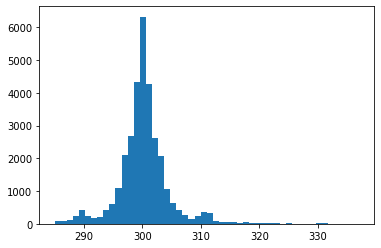

png

3.

(a)

python

res = df.Radiation.rolling('6H').corr(df.Temperature)
res.tail(3)

Datetime
2016-12-31 23:45:04    0.328574
2016-12-31 23:50:03    0.261883
2016-12-31 23:55:01    0.262406
dtype: float64

(b)

python

res = df.Temperature.resample('6H', origin='03:00:00').mean()
res.head(3)

Datetime
2016-08-31 21:00:00    51.218750
2016-09-01 03:00:00    50.033333
2016-09-01 09:00:00    59.379310
Freq: 6H, Name: Temperature, dtype: float64

(c)

python

my_dt = df.index.shift(freq='-6H')
int_loc = [df.index.get_indexer([i], method='nearest') for i in my_dt]
int_loc = np.array(int_loc).reshape(-1)
res = df.Radiation.iloc[int_loc]
res.index = df.index
res.tail(3)

Datetime
2016-12-31 23:45:04    9.33
2016-12-31 23:50:03    8.49
2016-12-31 23:55:01    5.84
Name: Radiation, dtype: float64

以及，纸质版中提到的另一种方法 merge_asof()，这个方法性能更好些。

python

target = pd.DataFrame(
    {
        "Time": df.index.shift(freq='-6H'),
        "Datetime": df.index,
    }
)
res = pd.merge_asof(
    target,
    df.reset_index().rename(columns={"Datetime": "Time"}),
    left_on="Time",
    right_on="Time",
    direction="nearest"
).set_index("Datetime").Radiation
res.tail(3)

Datetime
2016-12-31 23:45:04    9.33
2016-12-31 23:50:03    8.49
2016-12-31 23:55:01    5.84
Name: Radiation, dtype: float64

Ex2：水果销量数据集

1.

(a)

python

df = pd.read_csv('../data/fruit.csv')
df.Date = pd.to_datetime(df.Date)
df_grape = df.query("Fruit == 'Grape'")
res = df_grape.groupby([np.where(df_grape.Date.dt.day<=15,'First', 'Second'),
                        df_grape.Date.dt.month])['Sale'].mean().to_frame().unstack(0).droplevel(0,axis=1)
res = (res.First/res.Second).rename_axis('Month')
res.head()

Month
1    1.174998
2    0.968890
3    0.951351
4    1.020797
5    0.931061
dtype: float64

(b)

python

df[df.Date.dt.is_month_end].query("Fruit == 'Pear'").groupby('Date').Sale.sum().head()

Date
2019-01-31    847
2019-02-28    774
2019-03-31    761
2019-04-30    648
2019-05-31    616
Name: Sale, dtype: int64

(c)

python

df[df.Date.isin(pd.date_range('20190101', '20191231',freq='BM'))].query("Fruit == 'Pear'").groupby('Date').Sale.mean().head()

Date
2019-01-31    60.500000
2019-02-28    59.538462
2019-03-29    56.666667
2019-04-30    64.800000
2019-05-31    61.600000
Name: Sale, dtype: float64

(d)

python

target_dt = df.drop_duplicates().groupby(df.Date.drop_duplicates().dt.month)['Date'].nlargest(5).reset_index(drop=True)
res = df.set_index('Date').loc[target_dt].reset_index().query("Fruit == 'Apple'")
res = res.groupby(res.Date.dt.month)['Sale'].mean().rename_axis('Month')
res.head()

Month
1    65.313725
2    54.061538
3    59.325581
4    65.795455
5    57.465116
Name: Sale, dtype: float64

2.

python

month_order = ['January','February','March','April','May','June','July','August','September','October','November','December']
week_order = ['Mon','Tue','Wed','Thu','Fri','Sat','Sum']
group1 = df.Date.dt.month_name().astype('category').cat.reorder_categories(month_order, ordered=True)
group2 = df.Fruit
group3 = df.Date.dt.dayofweek.replace(dict(zip(range(7),week_order))).astype('category').cat.reorder_categories(week_order, ordered=True)
res = df.groupby([group1, group2,group3])['Sale'].count().to_frame().unstack(0).droplevel(0,axis=1)
res.head()

	Date	January	February	March	April	May	June	July	August	September	October	November	December
Fruit	Date
Apple	Mon	46	43	43	47	43	40	41	38	59	42	39	45
	Tue	50	40	44	52	46	39	50	42	40	57	47	47
	Wed	50	47	37	43	39	39	58	43	35	46	47	38
	Thu	45	35	31	47	58	33	52	44	36	63	37	40
	Fri	32	33	52	31	46	38	37	48	34	37	46	41

3.

python

df_apple = df[(df.Fruit=='Apple')&(~df.Date.dt.dayofweek.isin([5,6]))]
s = pd.Series(df_apple.Sale.values,index=df_apple.Date).groupby('Date').sum()
res = s.rolling('10D').mean().reindex(pd.date_range('20190101','20191231')).fillna(method='ffill')
res.head()

2019-01-01    189.000000
2019-01-02    335.500000
2019-01-03    520.333333
2019-01-04    527.750000
2019-01-05    527.750000
Freq: D, dtype: float64

参考答案 ​

第一章 预备知识 ​

Ex1：利用列表推导式写矩阵乘法 ​

Ex2：更新矩阵 ​

Ex3：卡方统计量 ​

Ex4：改进矩阵计算的性能 ​

Ex5：连续整数的最大长度 ​

第二章 pandas基础 ​

Ex1：口袋妖怪数据集 ​

1. ​

2. ​

3. ​

Ex2：指数加权窗口 ​

1. ​

2. ​

第三章 索引 ​

Ex1：公司员工数据集 ​

1. ​

2. ​

3. ​

Ex2：巧克力数据集 ​

1. ​

2. ​

3. ​

第四章 分组 ​

Ex1：汽车数据集 ​

1. ​

2. ​

3. ​

4. ​

5. ​

Ex2：实现transform函数 ​

第五章 变形 ​

Ex1：美国非法药物数据集 ​

1. ​

2. ​

3. ​

Ex2：特殊的wide_to_long方法 ​

第六章 连接 ​

Ex1：美国疫情数据集 ​

Ex2：实现join函数 ​

第七章 缺失数据 ​

Ex1：缺失值与类别的相关性检验 ​

Ex2：用回归模型解决分类问题 ​

1. ​

2. ​

第八章 文本数据 ​

Ex1：房屋信息数据集 ​

1. ​

2. ​

3. ​

Ex2：《权力的游戏》剧本数据集 ​

1. ​

2. ​

3. ​

第九章 分类数据 ​

Ex1：统计未出现的类别 ​

Ex2：钻石数据集 ​

1. ​

2. ​

3. ​

4. ​

5. ​

6. ​

第十章 时序数据 ​

Ex1：太阳辐射数据集 ​

1. ​

2. ​

3. ​

Ex2：水果销量数据集 ​

1. ​

2. ​

3. ​

参考答案

第一章预备知识

Ex1：利用列表推导式写矩阵乘法

Ex2：更新矩阵

Ex3：卡方统计量

Ex4：改进矩阵计算的性能

Ex5：连续整数的最大长度

第二章 pandas基础

Ex1：口袋妖怪数据集

1.

2.

3.

Ex2：指数加权窗口

1.

2.

第三章索引

Ex1：公司员工数据集

1.

2.

3.

Ex2：巧克力数据集

1.

2.

3.

第四章分组

Ex1：汽车数据集

1.

2.

3.

4.

5.

Ex2：实现transform函数

第五章变形

Ex1：美国非法药物数据集

1.

2.

3.

Ex2：特殊的wide_to_long方法

第六章连接

Ex1：美国疫情数据集

Ex2：实现join函数

第七章缺失数据

Ex1：缺失值与类别的相关性检验

Ex2：用回归模型解决分类问题

1.

2.

第八章文本数据

Ex1：房屋信息数据集

1.

2.

3.

Ex2：《权力的游戏》剧本数据集

1.

2.

3.

第九章分类数据

Ex1：统计未出现的类别

Ex2：钻石数据集

1.

2.

3.

4.

5.

6.

第十章时序数据

Ex1：太阳辐射数据集

1.

2.

3.

Ex2：水果销量数据集

1.

2.

3.